V1.00 22-Oct-01
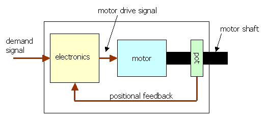
A "position demand" signal is detected by the control electronics. This signal represents a required position for the motor shaft to be in. The potentiometer attached to the shaft is used to tell the electronics where the motor shaft actually is. If there is a difference between the actual position and the demand position, then the electronics drives the motor in the appropriate direction to reduce that difference. The difference is called the "error signal", E, in control theory parlance.
E = Pa - Pd
E = Error signal
Pa = actual position
Pd = Demand position
The strength at which the motor is driven to reduce the error signal depends on how large the error signal is. If the error is large, then the motor must be driven hard and quick to reduce it. If the error is small, then the motor will only require a small push to reduce the error to nothing. Therefore, the strength of the motor drive signal is proportional to the error signal.
Vm = G x E
Vm = Motor drive level
E = Error signal
G = constant of proportionality.
The 'G' in this equation is the gain of the electronic circuit that detects the error signal and drives the motor.
Here is a control block diagram of the system with these signal names shown:
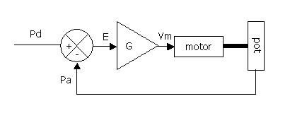
The circle with a cross in it is a summing junction (in this case the lower entry point to it is negated first, so it is a subtracting junction). The triangle is the amplifier with gain G.
So why don't we drive the motor at full power all the time? That is, why don't we make 'G' in the above equation very high, or even infinite (the amplifier output will saturate at the positive or negative power rail if the gain is very high)?
Imagine this experiment. You are sitting at a desk. Along the other side of the desk is a bank of lights, stretching from the left hand side right over to the right hand side. These lights are lit at random, one at a time, and your job is to point to the light that is lit as quickly as possible, with your arm straight and outstretched.

(apologies for the picture, you
get the idea!)
The amount of muscle power you require to point to the next light as quickly as possible will depend on how far away the next light is from the one you are currently pointing at. If the next light is next door to the one you are currently pointing at, you only require a little muscle power to move your arm. If, however, you are pointing to the leftmost light and the rightmost one is the next to be lit, you will need much more muscle power to swing your arm over as quickly as possible. As you get near to the new light, you will reduce the muscle power to make sure that you don't overshoot it. This is the same as the description above, where the amount of motor power required is proportional to the difference between the actual and the required positions.
So now can you imagine what would happen if you applied the maximum muscle power regardless of how far away the next light is? If the next light was next door to the current one, you would swing your arm over as hard as possible, and completely overshoot it. Then you must swing your arm back the other way again to compensate, but you will overcompensate, and your arm will overshoot in the other direction. In fact you will just end up swinging your arm back and forth wildly and never get to the required position. This is exactly what happens in a control application where the gain of the system is too high - it oscillates, and is unstable.
Now what would happen if you only applied a very small muscle force? You would have trouble keeping track of the lights - you would always be lagging behind the movement.
At some point in between these situations, you will be applying just the right amount of force so that as your arm swung over to the light, it would slow down and finish pointing right at the correct spot.
In control theory, these three situations are called "underdamped", "overdamped", and "critically damped".
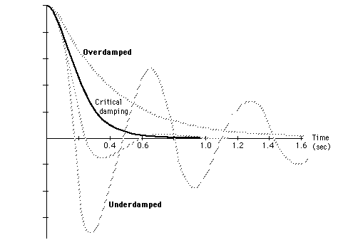
In fact the first situation is an extreme case of underdamping - instability - where the waveform doesn't die away as in the graph above, but continues to oscillate forever with the same amplitude.
The solution is to build a circuit where the gain is variable with a simple single knob-potentiometer, like the volume control on a hi-fi amplifier. Then we can experimentally adjust the gain until the system operates exactly how we want it too. If necessary, the gain potentiometer could then be replaced with a fixed value resistor.
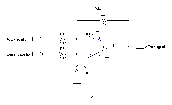
I'll go through the control block digram shown in section 2 above part by part and present designs for each section.
E = Pa - Pd
E = Error signal
Pa = actual position
Pd = Demand position
We also want to negate the value of the demand position. A suitable circuit is shown below:
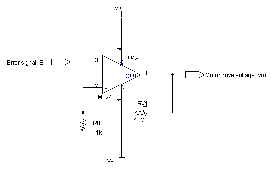
If more gain is required, this circuit can be fitted with a fixed 1M feedback resistor, and another identical section added with the variable 1M resistor. This would then allow the gain to be adjusted between 1000 and 1,000,000.
Alternatively, the motor can be placed between two L149s driven in anti- phase in a bridge configuration:
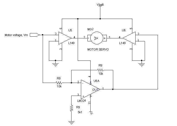
In this circuit, the LM324 U6a is used to invert the drive signal which then drives the right hand L149. Therefore, the motor left hand terminal sees a voltage Vm, and the right hand terminal -Vm, and so the voltage across the motor is
Vm - (-Vm) = 2Vm
The PWM must be generated by a voltage to PWM converter circuit, an example of which is presented in the PWM Generators page using the SG3525. The complete circuit is shown below:
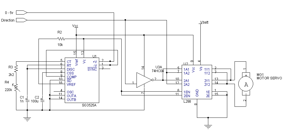 Click on the circuit diagram to open it in a new window.
Note that this is not striclty as "single-chip" solution, but the motor driver section is just one chip rather than a speed controller made up of discrete transistors.
Short circuit protection can be added to this circuit quite easily. The motor current goes through pins 1 and 15 of the L298 (which are tied straight to ground in the diagram above). If a sense resistor is placed here, a comparator can be used to compare the voltage with a reference value. The SG3525 output can be disabled by taking the SD (pin 10) input high.
The inputs to this circuit are an analogue (0 to 5 volts) speed demand signal, and a logic level direction signal. The logic direction signal can be generated by the error amplifier - it is effectivel just the sign of the error signal (+ve or -ve).
A circuit for generating a demand and a direction signal pair from a bipolar (-ve & +ve) input signal is presented in the Speed & Direction circuits.
An application note including PWM driving of the L298N is available from ST here.
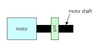
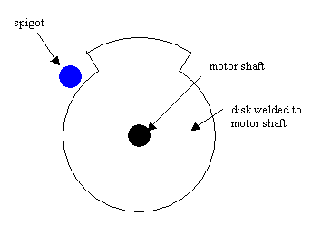
This method can only be used if the motor shaft is quite thin, and the pot can be threaded onto the motor shaft. The pot must be of a suitable kind (without a knob shaft) designed for mounting onto shafts.
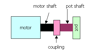
In this method, the potentiometer is mounted on the end of the motor shaft. This can only be done if the load is not attached to the end of course. The load may be driven off a gear wheel which is fitted further up the motor shaft.
There may be some non-alignment in the axis of the potentiometer shaft and the motor shaft. In this case, an Oldham coupling would make a suitable joint between the two.
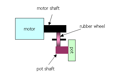
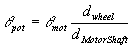
This may be the easiest method. A rubber wheel is mounted pressing up against the motor shaft such that it turns when the motor shaft turns. The ratio between the diameter of the motor shaft and the wheel will determine how the angle of the motor shaft varies with the angle of the potentiometer according to the following equation:
Drive the servo with a mid-point signal, and see what happens. The motor may not move at all. Gradually turn up the gain until the motor moves. If the motor starts spinning back and forth (oscillating), then the gain is too high. When the motor appears to have moved into the midpoint position, change the demand to one extreme, and make sure the motor moves to its endstop. Now move the demand to the other extreme, and the motor should move to its other endstop. If the motor does not move far enough, the gain may be set too low.
When the servo is fixed in the robot, and the motor is driving a load, then it is possible that the gain may need to be increased to overcome the frictional force of the load.
Once a suitable gain setting has been found, the gain pot may be replaced with a fixed resistor, or better still, a dob of hot-melt glue dripped onto it to stop it moving due to vibration. This will allow the setting to be changed if necessary.
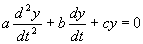
y is the position of the object at a point in time. The three coefficients, a, b, and c, determine the motion of the object under these conditions. The first coefficient, a, is a measure of the springiness in the system, the second coefficient, b, is a measure of the damping in the system, and the third coefficient, c, is the mass of the object. a and c determine the frequency of oscillation, and b determines the rate at which the oscillation decays.
Servo motor stability and step response.
| Manufacturer | Device |
| SGS Thompson | SG3525A SMPS controller |
| L298N Motor controller | |
| L149 Power Opamp | |
| LM324 Quad signal opamp | |
74HC04 Hex inverter |
[E5] A basic introduction to radio control servos
http://www.seattlerobotics.org/guide/servos.html
[E3] Explanations of simple harmonic motion, oscillations, and damping.
http://230nsc1.phy-astr.gsu.edu/hbase/shm.html#c1
http://webug.physics.uiuc.edu/courses/phys225/fall01/lectures/oscillations/sld001.htm
[E2] A set of slides describing wheel positioning servo systems for robots
http://www-robotics.usc.edu/~gaurav/CS547/MobileRobotDynamicsControl/sld020.htm