This page examines in detail the electrical engineering and control theory behind the operation of the DC motor servo, and derives an equation for the stability of the system. It is quite advanced, and uses the theories listed below. I do not present any introduction to these theories since that would make this page thousands of lines long. I can only suggest you perform web searches on the areas involved if you want to know more about them. I have appended a bibliography also that I used to develop this page.
Theories involved:
I have recreated the servo system in the first diagram on the main power servo page here:
In this block diagram, I have represented the DC motor and the potentiometer attached to its shaft as the transfer function G(s), and the amplifier with gain A. We will determine what the allowable range of A is to keep the system stable. The input of G(s) is the armature voltage of the motor, ea, and its output is the motor shaft angular position, θm.
From the block diagram,

The closed loop transfer function of this system is
Let’s see what the equation for G(s) actually is using DC machine theory:
The parameters shown are:
The torque is proportional to current in a permanent magnet DC motor, so

The torque of the load is made up of the moment of inertia of the load, and the frictional force of the load, and is given by the equation
The back emf is proportional to the flux and to the speed, and since the flux is constant in a permanent magnet machine:
Kirchoff’s law around the armature circuit gives us:
Combining all these equations gives us
Since the angular speed, ωm, is the rate of change of angle:

Using the Laplace variable notation, where multiplying by s represents differentiation in time:

Then:
replacing the values in square brackets with variables:
From before:
So the system transfer function is
The characteristic equation which determines system stability is
It is a necessary (but not sufficient) condition of system stability that all the coefficients of this equation must be the same sign.
We enter these coefficients into the Routh array:
s3: |
ao |
a2 |
s2: |
a1 |
A |
s: |
|
|
const: |
A |
|
The other condition of system stability is that all the elements in the first column are the same sign. Since a0 and a1 are always positive (from their definitions), then

must also be positive. Therefore

Expanding the variables:
It is obvious that A must be positive for stability, since a negative gain would make the servo mechanism compensate for any positional error by driving the motor the wrong way.
Several of these quantities are rather hard to calculate or measure in practice - that is why the circuit in the power servos section has a variable gain which is set empirically.
Notice that as the inductance of the motor is reduced, the gain may be increased - it is only the inductance of the motor that limits the gain and may make the system unstable. If the inductance was zero (which in practice it never can be), then there would be no limit on the positive value of the gain.
We can now calculate the response of the servo mechanism to a step change in position demand signal. Without going through any proofs, if the system closed loop transfer function is:
then the step response for an underdamped system is
where

equating this transfer function with the TF we generated:
The value ζ is the damping factor, and determines the type of response, underdamped (ζ<1), critically damped (ζ=1), or overdamped (ζ>1).
We can now plot the response based on the values of a1 and a2 (which are in turn based on the system and motor parameters). For the values shown:
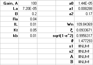
This is the response:
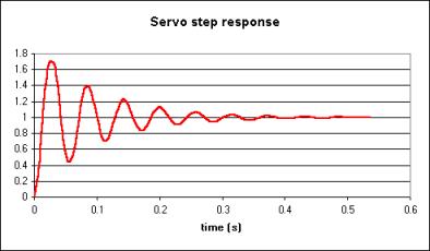
The step response for an overdamped system is given by the equation:
By increasing the frictional load, B, we can simulate the system become overdamped. For example, changing the value of B from 0.2 to 4 gives the following response:
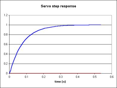
The spreadsheet used to generate these graphs is available here in MS Excel 4.0 format. This spreadheet graphs underdamped and overdamped systems. Depending on the system being displayed, the cells for the other type of system may have the value "#NUM" indicating that the square root of a negative number is present, which is to be expected.
Introduction to control theory.
S.A. Marshall
Macmillan
ISBN 0 333 18312 6
Feedback control system analysis and synthesis. 2nd ed.
J.J. D'Azzo and C.H. Houpis
McGraw Hill
Both these books are now deleted, but the latter's new version is...
Linear Control System Analysis and Design
J.J. D'Azzo and C.H. Houpis
McGraw Hill
ISBN 0 070 16321 9